.ipynb .pdf

open issue

Binder Live Code

Contents

Spatial Interpolation - Part 2

Analysis Preparation

Imports

All of these libraries should have been previously installed during the environment set-up, if they have not been installed already you can use install.packages(c("raster", "rgdal", "ape", "scales", "deldir", "gstat"))

library(raster) # rasters
library(rgdal)  # spatial data
library(sf)     # for handling spatial features
library(ape)    # clustering (Morans I)
library(scales) # transparencies
library(deldir) # triangulation
library(gstat)  # geostatistics

source('../scripts/helpers.R') # helper script, note that '../' is used to change into the directory above the directory this notebook is in

Loading required package: sp

rgdal: version: 1.5-16, (SVN revision 1050)
Geospatial Data Abstraction Library extensions to R successfully loaded
Loaded GDAL runtime: GDAL 3.1.4, released 2020/10/20
Path to GDAL shared files: /srv/conda/envs/notebook/share/gdal
GDAL binary built with GEOS: TRUE 
Loaded PROJ runtime: Rel. 7.1.1, September 1st, 2020, [PJ_VERSION: 711]
Path to PROJ shared files: /srv/conda/envs/notebook/share/proj
PROJ CDN enabled: TRUE
Linking to sp version:1.4-2
To mute warnings of possible GDAL/OSR exportToProj4() degradation,
use options("rgdal_show_exportToProj4_warnings"="none") before loading rgdal.

Linking to GEOS 3.8.1, GDAL 3.1.4, PROJ 7.1.1


Attaching package: ‘ape’


The following objects are masked from ‘package:raster’:

    rotate, zoom


deldir 0.2-3      Nickname: "Stack Smashing Detected"


     Note 1: As of version 0.2-1, error handling in this 
     package was amended to conform to the usual R protocol. 
     The deldir() function now actually throws an error 
     when one occurs, rather than displaying an error number 
     and returning a NULL.
 
     Note 2:  As of version 0.1-29 the arguments "col" 
     and "lty" of plot.deldir() had their names changed to 
     "cmpnt_col" and "cmpnt_lty" respectively basically 
     to allow "col" and and "lty" to be passed as "..." 
     arguments.
 
     Note 3: As of version 0.1-29 the "plotit" argument 
     of deldir() was changed to (simply) "plot".
 
     See the help for deldir() and plot.deldir().

Loading Data

We’ll start by again checking to see if we need to download any data.

download_data()

We’ll then load in the datasets.

df_zambia <- read_sf('../data/zambia/zambia.shp')
df_africa_cities <- read_sf('../data/africa/cities.shp')
solar <- raster('../data/zambia/solar.tif')
altitude <- raster('../data/zambia/altitude.tif')

Do some pre-processing on the zambian cities dataset (which we’ll use as points in our Voronoi diagram later).

df_zambian_cities <- df_africa_cities[which(df_africa_cities$COUNTRY=='Zambia'), ]
df_zambian_cities_UTM35S <- st_transform(df_zambian_cities, crs=st_crs(20935))

head(df_zambian_cities_UTM35S, 3)

A sf: 3 × 29

LATLONGID	LATITUDE	LONGITUDE	URBORRUR	YEAR	ES90POP	ES95POP	ES00POP	INSGRUSED	CONTINENT	geometry	⋯	SCHADMNM	ADMNM1	ADMNM2	TYPE	SRCTYP	COORDSRCE	DATSRC	LOCNDATSRC	NOTES	geometry
<dbl>	<dbl>	<dbl>	<chr>	<dbl>	<int>	<int>	<int>	<chr>	<chr>	⋯	<chr>	<chr>	<chr>	<chr>	<chr>	<chr>	<chr>	<chr>	<chr>	<POINT [m]>
4	-12.65000	28.08333	U	1990	9945	10684	11218	N	Africa	POINT (617646.2 8601614)	⋯	COPPERBELT	Copperbelt	Kalulushi	UA	Published	NIMA	Census of Population, Housing & Argriculture 1990 Descriptive Tables	UN Statistical Library	NA	POINT (617646.2 8601614)
7	-12.36667	27.83333	U	1990	48055	51629	54206	N	Africa	POINT (590593.6 8633048)	⋯	COPPERBELT	Copperbelt	Chililabombwe	UA	Published	NIMA	Census of Population, Housing & Argriculture 1990 Descriptive Tables	UN Statistical Library	NA	POINT (590593.6 8633048)
9	-12.53333	27.85000	U	1990	142383	152972	160610	N	Africa	POINT (592346.6 8614610)	⋯	COPPERBELT	Copperbelt	Chingola	UA	Published	NIMA	Census of Population, Housing & Argriculture 1990 Descriptive Tables	UN Statistical Library	NA	POINT (592346.6 8614610)

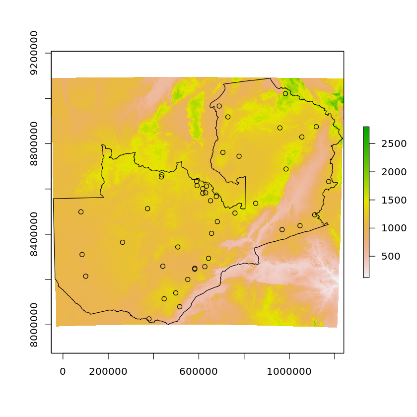
We’ll visualise these as well

plot(altitude)
plot(df_zambia['geometry'], add=TRUE)
plot(df_zambian_cities_UTM35S['geometry'], add=TRUE)

Interpolation

First we’ll extract the solar and altitude values for the points we’ve selected (just so happens to be cities in this case).

city_coords = st_coordinates(df_zambian_cities_UTM35S)

df_zambian_cities_UTM35S$solar <- extract(solar, city_coords)
df_zambian_cities_UTM35S$altitude <- extract(altitude, city_coords)

df_zambian_cities_UTM35S$x <- city_coords[, 1]
df_zambian_cities_UTM35S$y <- city_coords[, 2]

We’ll now create a grid that we will carry out the predictions over

grid <- st_as_sf(rasterToPoints(solar, spatial=TRUE)) # uses existing raster cell centres as point locations
grid$solar <- NULL # clear existing data

plot(grid, pch=".")

idw <- gstat::idw(solar~x+y, df_zambian_cities_UTM35S, newdata= grid)

Error in .local(formula, locations, ...): stars required: install that first
Traceback:

1. gstat::idw(solar ~ x + y, df_zambian_cities_UTM35S, newdata = grid)
2. gstat::idw(solar ~ x + y, df_zambian_cities_UTM35S, newdata = grid)
3. .local(formula, locations, ...)
4. stop("stars required: install that first")

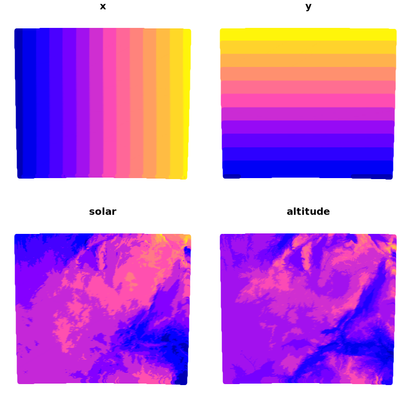
We’ll now populate this empty grid with the x/y values and solar/altitude values

grid_coords <- as.data.frame(st_coordinates(grid))

grid$x <- grid_coords[, 1]
grid$y <- grid_coords[, 2]

grid$solar <- extract(solar, grid_coords[, 1:2])
grid$altitude <- extract(altitude, grid_coords[, 1:2])

plot(grid)

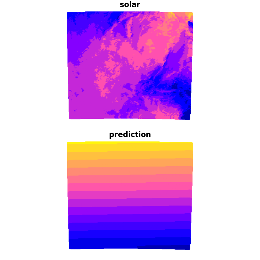
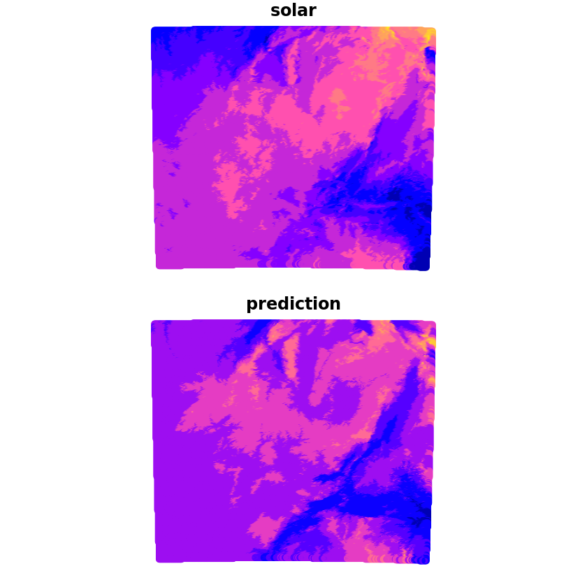
We can now make the prediction which we’ll compare with the true solar values, we can see that whilst it captures some of the wider characteristics there are a lot of discrepancies still.

grid_pred <- predict(trend_1st, newdata=grid, se.fit=TRUE)
grid$prediction <- grid_pred$fit

plot(grid[c('solar', 'prediction')])

We don’t just have to regress against longitude/latitude though, here we’ll repeat the previous steps but only use latitude as a regressor.

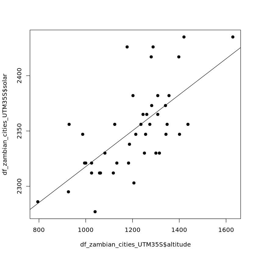
First we’ll visualise the relationship between the two.

plot(df_zambian_cities_UTM35S$altitude, df_zambian_cities_UTM35S$solar, pch=19)
abline(lm(df_zambian_cities_UTM35S$solar ~ df_zambian_cities_UTM35S$altitude))

Then we’ll fit a model and use it in our prediction.

trend_1st <- lm(solar~altitude, data=df_zambian_cities_UTM35S)

grid_pred <- predict(trend_1st, newdata=grid, se.fit=TRUE)
grid$prediction <- grid_pred$fit

plot(grid[c('solar', 'prediction')])

Questions

Best Fit Model

• What combination of the inputs produces the most accurate results?

• Should we use the standard r2 score or the adjusted r2 score?

• How do the results change when you use a test/train split?

• How could we improve over a random sample on the test/train split? (Think about what you would do with time-series cross-validation)

# 

previous

Spatial Interpolation - Part 1

next

Coursework Support